JAXA Virtual Planet: Quick Guide

JAXA Virtual Planet (VP) is a web-based GIS for exploring and analyzing lunar datasets from Kaguya. There is an “Basic” mode for the general public, and an “Advanced” mode for researchers which features enhanced analytical functions.

VP demo — This figure shows an example of layers displayed via JAXA Virtual Planet. This example shows feature names over the lunar global topography layer.

About JAXA Virtual Planet (VP)

VP has an Basic mode (high-operability system for the general public) and an Advanced mode (system with sophisticated analytical functions for researchers). They can be accessed at the URLs below.

Access URLs

Select a mode based on what you want to do.

Mode	Purpose	URL
Basic	Data browsing	https://vp.darts.isas.jaxa.jp/moon/?lang=en
Advanced	Data analysis	https://vp.darts.isas.jaxa.jp/moon/?lang=en&pro=1

*Analyses can be performed by displaying the layer containing the necessary information and using the tools included in the toolbox, after first selecting a mode and a view to display.

Available views

Mode	View	Coordinate System (Click to show WKT)
Basic/Advanced	3D globe	GCS_Moon_2000 (ESRI:104903) `GEOGCS["GCS_Moon_2000",DATUM["D_Moon_2000",SPHEROID["Moon_2000_IAU_IAG",1737400.0,0.0]],PRIMEM["Reference_Meridian",0.0],UNIT["Degree",0.0174532925199433]]`
Basic/Advanced	Equidistant cylindrical 3D	SIMPLE_CYLINDRICAL_MOON `PROJCS["SIMPLE_CYLINDRICAL_MOON",GEOGCS["GCS_MOON",DATUM["D_MOON",SPHEROID["MOON",1737400.0,0.0]],PRIMEM["Reference_Meridian",0.0],UNIT["Degree",0.0174532925199433]],PROJECTION["Plate_Carree"],PARAMETER["false_easting",0.0],PARAMETER["false_northing",0.0],PARAMETER["central_meridian",0.0],UNIT["Meter",1.0]]`
Basic/Advanced	North polar stereographic 3D	PolarStereographic_Moon (Stereographic_North_Pole) `PROJCS["PolarStereographic_Moon",GEOGCS["GCS_Moon",DATUM["D_Moon",SPHEROID["Moon_polarRadius",1737400.0,0.0]],PRIMEM["Reference_Meridian",0.0],UNIT["Degree",0.0174532925199433]],PROJECTION["Stereographic_North_Pole"],PARAMETER["false_easting",0.0],PARAMETER["false_northing",0.0],PARAMETER["central_meridian",0.0],PARAMETER["standard_parallel_1",90.0],UNIT["Meter",1.0]]`
Basic/Advanced	South polar stereographic 3D	PolarStereographic_Moon (Stereographic_South_Pole) `PROJCS["PolarStereographic_Moon",GEOGCS["GCS_Moon",DATUM["D_Moon",SPHEROID["Moon_polarRadius",1737400.0,0.0]],PRIMEM["Reference_Meridian",0.0],UNIT["Degree",0.0174532925199433]],PROJECTION["Stereographic_South_Pole"],PARAMETER["false_easting",0.0],PARAMETER["false_northing",0.0],PARAMETER["central_meridian",0.0],PARAMETER["standard_parallel_1",-90.0],UNIT["Meter",1.0]]`
Advanced only	Equidistant cylindrical 2D	SIMPLE_CYLINDRICAL_MOON `PROJCS["SIMPLE_CYLINDRICAL_MOON",GEOGCS["GCS_MOON",DATUM["D_MOON",SPHEROID["MOON",1737400.0,0.0]],PRIMEM["Reference_Meridian",0.0],UNIT["Degree",0.0174532925199433]],PROJECTION["Plate_Carree"],PARAMETER["false_easting",0.0],PARAMETER["false_northing",0.0],PARAMETER["central_meridian",0.0],UNIT["Meter",1.0]]`
Advanced only	North polar stereographic 2D	PolarStereographic_Moon (Stereographic_North_Pole) `PROJCS["PolarStereographic_Moon",GEOGCS["GCS_Moon",DATUM["D_Moon",SPHEROID["Moon_polarRadius",1737400.0,0.0]],PRIMEM["Reference_Meridian",0.0],UNIT["Degree",0.0174532925199433]],PROJECTION["Stereographic_North_Pole"],PARAMETER["false_easting",0.0],PARAMETER["false_northing",0.0],PARAMETER["central_meridian",0.0],PARAMETER["standard_parallel_1",90.0],UNIT["Meter",1.0]]`
Advanced only	South polar stereographic 2D	PolarStereographic_Moon (Stereographic_South_Pole) `PROJCS["PolarStereographic_Moon",GEOGCS["GCS_Moon",DATUM["D_Moon",SPHEROID["Moon_polarRadius",1737400.0,0.0]],PRIMEM["Reference_Meridian",0.0],UNIT["Degree",0.0174532925199433]],PROJECTION["Stereographic_South_Pole"],PARAMETER["false_easting",0.0],PARAMETER["false_northing",0.0],PARAMETER["central_meridian",0.0],PARAMETER["standard_parallel_1",-90.0],UNIT["Meter",1.0]]`

Displayable layers

The following layers are available. Initially, only the base map is displayed.

See the links below for source data and references.

Layer information (Click to expand)

Layer name Detailed description

Nomenclature Lunar nomenclature is cited from the USGS Gazetteer of Planetary Nomenclature.

Graticule

The geographic coordinate system is based on GCS_Moon_2000 (ESRI:104903).

WKT


                      GEOGCS["GCS_Moon_2000",DATUM["D_Moon_2000",SPHEROID["Moon_2000_IAU_IAG",1737400.0,0.0]],PRIMEM["Reference_Meridian",0.0],UNIT["Degree",0.0174532925199433]]

Lunar global topography

Lunar global topography [km] map acquired by SELENE Laser Altimeter (LALT) observations. The product is represented by 360-degree spherical harmonics referenced to a 1737.4 km sphere at the lunar center of mass. For an overview of the instrument, see below:
https://www.kaguya.jaxa.jp/en/equipment/lalt_e.htm
Data source:
https://data.darts.isas.jaxa.jp/pub/pds3/sln-l-lalt-5-topo-ggt-map-v2.0/
https://data.darts.isas.jaxa.jp/pub/pds3/sln-l-lalt-5-topo-gt-np-img-v2.0/
https://data.darts.isas.jaxa.jp/pub/pds3/sln-l-lalt-5-topo-gt-sp-img-v2.0/

References

This data should be cited as follows when used in papers, etc.:
Araki, H., Tazawa, S., Ishihara, Y., et al. Lunar global shape and polar topography derived from Kaguya-LALT laser altimetry. Science, 323, 5916, 897-900 (2009). https://doi.org/10.1126/science.1164146

Mare unit age

Polygons representing the estimated ages [Gyr] of lunar maria based on stratigraphic relationships of mare basalt units interpreted from SELENE Lunar Radar Sounder (LRS). The source data were obtained from Figure 5 in Oshigami et al. (2014). The absolute ages were determined based on crater size–frequency distributions reported in Hiesinger et al. (2000, 2003, 2010), Kodama and Yamaguchi (2003), and Morota et al. (2011).

References

Oshigami, S., Watanabe, S., Yamaguchi, Y., et al. Mare volcanism: Reinterpretation based on Kaguya Lunar Radar Sounder data. Journal of Geophysical Research Planets, 119, 1037–1045 (2014). https://doi.org/10.1002/2013JE004568
Hiesinger, H., Jaumann, R., Neukum, G., et al. Ages of mare basalts on the lunar nearside. Journal of Geophysical Research Planets, 105, 29229–29275 (2000). https://doi.org/10.1029/2000JE001244
Hiesinger, H., Head III, J. W., Wolf, U., et al. Ages and stratigraphy of mare basalts in Oceanus Procellarum, Mare Nubium, Mare Cognitum, and Mare Insularum. Journal of Geophysical Research Planets, 108, E7, 5065 (2003). https://doi.org/10.1029/2002JE001985
Morota, T., Haruyama, J., Ohtake, M., et al. Timing and characteristics of the latest mare eruption on the Moon. Earth and Planetary Science Letters, 302, 255–266 (2011). https://doi.org/10.1016/j.epsl.2010.12.028
Kodama, S., and Yamaguchi, Y. Lunar mare volcanism in the eastern nearside region derived from Clementine UV/VIS data. Meteoritics & Planetary Science 38, Nr 10, 1461–1484 (2003). https://doi.org/10.1111/j.1945-5100.2003.tb00251.x

LRS subsurface reflection points

The unit boundary depths of mare basalts determined by Ishiyama and Kumamoto (2019), based on radargrams obtained by SELENE Lunar Radar Sounder (LRS), are shown. By clicking on a point displayed in Mare Smythii, the depths of four echoes (i.e., unit boundaries) at that location are displayed. Elevation of surface indicates the depth of the surface echo read from the LRS radargram, Elevation of echo 1–4 indicate the depths of subsurface echoes read from the LRS data, Apparent depth is the difference between the surface echo and the subsurface echoes, and Depth is the true depth calculated assuming a dielectric constant of 6.

References

This data should be cited as follows when used in papers, etc.:
Ishiyama, K. and Kumamoto, A. Volcanic history in the Smythii basin on SELENE radar observation. Scientific Reports, 9, 14502 (2019). https://doi.org/10.1038/s41598-019-50296-9

SP radiance & diffuse reflectance

Hyperspectral visible and near-infrared reflectance spectra based on the SP Level2C Product derived from observations by the SELENE Spectral Profiler (SP). The SP acquired hyperspectral data over areas of ~500 m × 500 m across the Moon. By clicking on an observation point in this layer displays the radiance [W/m²/μ/Sr] and diffuse reflectance. Spectra from the VIS and NIR1 detectors are calibrated following Yokota et al. (2011), and the NIR2 detector is calibrated following Yamamoto et al. (2014). The "thinned" layer achieves faster rendering by reducing the number of full observation points. For faster loading, the 2D view is recommended over the 3D view.
For an overview of the instrument, see below:
https://www.kaguya.jaxa.jp/en/equipment/tc_e.htm
Data source:
https://data.darts.isas.jaxa.jp/pub/pds3/sln-l-sp-4-level2c-v3.0/

References

This data should be cited as follows when used in papers, etc.:
Yokota, Y., Matsunaga, T., Ohtake, M., et al. Lunar photometric properties at wavelengths 0.5-1.6 μm acquired by SELENE Spectral Profiler and their dependency on local albedo and latitudinal zones. Icarus, 215, 639-660 (2011). https://doi.org/10.1016/j.icarus.2011.07.028
Yamamoto, S., Matsunaga, T., Ogawa, Y., et al. Calibration of NIR 2 of Spectral Profiler onboard Kaguya/SELENE. IEEE Transactions on Geoscience and Remote Sensing, 52, 6882-6868 (2014). https://doi.org/10.1109/TGRS.2014.2304581

SAR data

A 2D subsurface cross-sectional image derived from reflection echoes acquired by the Kaguya Lunar Radar Sounder (LRS), processed using along-track synthetic aperture lengths of 5 km, 10 km, and 40 km. Clicking on a survey line displays the product. The horizontal axis represents the along-track direction of the spacecraft. The vertical axis shows the apparent depth calculated assuming a dielectric constant of ε = 1, which differs from the actual depth. Surface and subsurface discontinuities appear as variations in echo intensity. The spatial resolution is approximately 75 m in the horizontal direction and ~75 m in apparent depth on the vertical axis.
For an overview of the instrument, see below:
https://www.kaguya.jaxa.jp/en/equipment/lrs_e.htm
Data source:
5km: https://data.darts.isas.jaxa.jp/pub/pds3/sln-l-lrs-5-sndr-ss-sar05-power-v1.0/
10 km: https://data.darts.isas.jaxa.jp/pub/pds3/sln-l-lrs-5-sndr-ss-sar10-power-v1.0/
40 km: https://data.darts.isas.jaxa.jp/pub/pds3/sln-l-lrs-5-sndr-ss-sar40-power-v1.0/

References

Ono, T., Kumamoto, A., Kasahara, Y., et al. The Lunar Radar Sounder (LRS) Onboard the KAGUYA (SELENE) Spacecraft. Space Science Reviews, 154, 145-192 (2010). https://doi.org/10.1007/s11214-010-9673-8
This data should be cited as follows when used in papers, etc.:
Kobayashi, T., Kim, J. H., Lee, S. R., et al. Synthetic aperture radar processing of Kaguya Lunar Radar Sounder data for lunar subsurface imaging. IEEE Transactions on Geoscience and Remote Sensing, 50, 6082437, 2161-2174 (2012). https://doi.org/10.1109/TGRS.2011.2171349

LRS Radargram

2D high-resolution subsurface cross section of reflected echo intensity obtained by SELENE Lunar Radar Sounder (LRS). Clicking on a survey line displays the product. The horizontal axis is the satellite ground track. The vertical axis represents the apparent depth calculated with dielectric constant ε = 1, which differs from the actual depth. Surface and subsurface discontinuities appear as variations in echo intensity. The spatial resolution is ~75 m on the horizontal axis and ~75 m on the apparent depth of the vertical axis.
For an overview of the instrument, see below:
https://www.kaguya.jaxa.jp/en/equipment/lrs_e.htm
Data source:
https://data.darts.isas.jaxa.jp/pub/pds3/sln-l-lrs-5-sndr-ss-high-v2.0/

References

Ono, T., Kumamoto, A., Kasahara, Y., et al. The Lunar Radar Sounder (LRS) Onboard the KAGUYA (SELENE) Spacecraft. Space Science Reviews, 154, 145-192 (2010). https://doi.org/10.1007/s11214-010-9673-8

MI FeO & TiO₂ abundance

Abundance (wt%) of FeO and TiO₂ based on SELENE Multiband Imager (MI) observations. This product was calculated from the MI_MAP product using the method by Otake et al. (2012). This layer covers latitudes from 85°N to 85°S with a spatial resolution of 128 pix/degree.

References

This data should be cited as follows when used in papers, etc.:
Otake, H., M. Ohtake, and N. Hirata, Lunar iron and titanium abundance algorithms based on SELENE (Kaguya) Multiband Imager data, Lunar and Planetary Science Conference, 43rd (2012), Abstract 1905. https://ui.adsabs.harvard.edu/abs/2012LPI....43.1905O

MI reflectance

Visible and near-infrared reflectance spectral data based on the MI_MAP Product derived from observations by the SELENE Multiband Imager (MI). The MI_MAP product is a 9-band data cube covering latitudes from 85°N to 85°S with a spatial resolution of 2048 pix/degree. This layer allows viewing of the reflectance spectrum at a selected position by clicking. Two reflectance values are plotted at 1000 nm because this is observed by both the VIS and NIR detectors.
For an overview of the instrument, see below:
https://www.selene.jaxa.jp/en/equipment/tc_e.htm
Data source:
https://data.darts.isas.jaxa.jp/pub/pds3/sln-l-mi-5-map-v3.0/

References

Ohtake, M., Haruyama, J., Matsunaga, T., et al. Performance and scientific objectives of the SELENE (KAGUYA) Multiband Imager. Earth, Planets and Space 60, 257–264 (2008). https://doi.org/10.1186/BF03352789

GRS nuclide map

The mass concentration distribution of K [ppm], Th [ppm], U [ppm], and CaO [wt%] based on observations by the SELENE Gamma-Ray Spectrometer (GRS) at an altitude of ~100 km. The product covers the entire lunar surface with an intrinsic spatial resolution of ~150 km.
For an overview of the instrument, see below:
https://www.kaguya.jaxa.jp/en/equipment/grs_e.htm
Data source:
https://data.darts.isas.jaxa.jp/pub/pds3/sln-l-grs-5-nuclide-map-v1.0/

References

K [ppm]	Kobayashi, S., Hasebe, N., Shibamura, E., et al. Determining the absolute abundances of natural radioactive elements on the lunar surface by the Kaguya Gamma-ray Spectrometer. Space Science Reviews 154, 193–218 (2010). https://doi.org/10.1007/s11214-010-9650-2
Th [ppm]	Yamashita, N., Hasebe, N., Reedy, R.C., et al. Uranium on the Moon: Global distribution and U/Th ratio. Geophysical Research Letters 37, L10201 (2010). https://doi.org/10.1029/2010GL043061
U [ppm]	Yamashita, N., Hasebe, N., Reedy, R.C., et al. Uranium on the Moon: Global distribution and U/Th ratio. Geophysical Research Letters 37, L10201 (2010). https://doi.org/10.1029/2010GL043061
CaO [wt%]	Yamashita, N., Gasnault, O., Forni, O., et al. The global distribution of calcium on the Moon: Implications for high-Ca pyroxene in the eastern mare region. Earth and Planetary Science Letters 38, 93–98 (2012). https://doi.org/10.1016/j.epsl.2012.08.010

TC reflectance map (low Sun)

Surface reflectance map acquired by SELENE Terrain Camera (TC) under low solar illumination from the east (morning) and from the west (evening). This product covers most of the globe at a resolution of 10 m/pixel, except for some high-latitude areas longitudinal areas.
For an overview of the instrument, see below:
https://www.kaguya.jaxa.jp/en/equipment/tc_e.htm
Data source:
Morning: https://data.darts.isas.jaxa.jp/pub/pds3/sln-l-tc-5-morning-map-v4.0/
Evening: https://data.darts.isas.jaxa.jp/pub/pds3/sln-l-tc-5-evening-map-v4.0/

References

Haruyama, J., Ohtake, M., Matsunaga, T., et al. Data products of SELENE (Kaguya) Terrain Camera for future lunar missions. 45th Lunar and Planetary Science Conference, p. 1304 (2014). https://ui.adsabs.harvard.edu/abs/2014LPI....45.1304H

TC ortho map

TC ortho data acquired by SELENE Terrain Camera (TC). This product covers most of the globe at a resolution of 10 m/pixel, except for some high-latitude areas longitudinal areas.
For an overview of the instrument, see below:
https://www.kaguya.jaxa.jp/en/equipment/tc_e.htm
Data source:
https://data.darts.isas.jaxa.jp/pub/pds3/sln-l-tc-5-ortho-map-v2.0/

References

TC DTM (SLDEM2013)

DTM map based on the SLDEM2013 product which combined observations from the SELENE Terrain Camera (TC), Multiband Imager (MI), and NASA Lunar Orbiter Laser Altimeter (LOLA). The DTM was primarily generated from TC (10 m/pix), with gaps filled using MI (20 m/pix) and LOLA (60 m/pix). The product covers the entire Moon.
Data source:
https://data.darts.isas.jaxa.jp/pub/pds3/sln-l-tc-5-sldem2013-v1.0/

References

Bouguer gravity anomaly

Bouguer gravity anomaly [mGal] model based on the SGM100h lunar gravity field model with degree 100. The gravity model was derived from the 4-way Doppler observations using SELENE RSAT and VRAD Satellite. The bouguer gravity anomaly is calculated from SGM100h and a LALT topographic model (STM-359_grid-03) assuming the crustal density of 2800 kg/m³. The high-frequency “spotty” signatures are likely due to the less accurate gravity coefficients above degree 70.
For an overview of the instrument, see below:
https://www.kaguya.jaxa.jp/en/equipment/rsat_e.htm
Data source:
SGM100h grid data, RISE Project

References

This data should be cited as follows when used in papers, etc.:
Matsumoto, K., Goossens, S., Ishihara, Y., et al. An improved lunar gravity field model from SELENE and historical tracking data: Revealing the farside gravity features. Journal of Geophysical Research: Planets, 115, E06007 (2010), https://doi.org/10.1029/2009JE003499

Free air gravity anomaly

Bouguer gravity anomaly [mGal] model based on the SGM100h lunar gravity field model with degree 100. The gravity model was derived from the 4-way Doppler observations using SELENE RSAT and VRAD Satellite.
For an overview of the instrument, see below:
https://www.kaguya.jaxa.jp/en/equipment/rsat_e.htm
Data source:
https://data.darts.isas.jaxa.jp/pub/pds3/sln-l-rise-5-grav-map-v1.0/
SGM100h grid data, RISE Project

References

Crustal thickness

Lunar crustal thickness map derived from the SGM100h lunar gravity field model and STM-359_grid-03 lunar topography model. The gravity model was derived from the 4-way Doppler observations using SELENE RSAT and VRAD Satellite. The topography model is derived from SELENE LALT observations. This product was created with the condition that the Bouguer gravity anomaly is explained by Moho topography without having the mantle exposed at the lunar surface. Assumed densities of the crust, mantle, and mare basalt layer are 2800 kg/m³, 3360 kg/m³, and 3200 kg/m³, respectively.
Data source:
Grid data of crustal thickness model, RISE Project

References

This data should be cited as follows when used in papers, etc.:
Ishihara, Y., Goossens, S., Matsumoto, K., et al. Crustal thickness of the Moon: Implications for farside basin structures. Geophysical Research Letters, 36, L19202 (2009). https://doi.org/10.1029/2009GL039708

Magnetic anomaly

Lunar magnetic anomaly mosaic data acquired by SELENE Lunar Magnetometer (LMAG) observations at an altitude of 100 km. This product shows the components of the lunar magnetic anomaly vector (X: east–west; Y: north–south; Z: radial; F: total magnetic field intensity).
For an overview of the instrument, see below:
https://www.kaguya.jaxa.jp/en/equipment/lmag_e.htm
Data source:
https://data.darts.isas.jaxa.jp/pub/pds3/sln-l-lmag-5-ma-map-v1.0/

References

Magnetic anomaly OP

Lunar magnetic anomaly mosaic data derived from SELENE Lunar Magnetometer (LMAG) observations at an altitude of ~30 km. This product shows the components of the lunar magnetic anomaly vector (X: east–west component; Y: north–south component; Z: radial component; F: total magnetic field intensity).
For an overview of the instrument, see below:
https://www.kaguya.jaxa.jp/en/equipment/lmag_e.htm
Data source:
https://data.darts.isas.jaxa.jp/pub/pds3/sln-l-lmag-5-ma-map-option-v1.0/

References

Tsunakawa, H., Shibuya, H., Takahashi, F., et al. Lunar magnetic field observation and initial global mapping of lunar magnetic anomalies by MAP-LMAG onboard SELENE (Kaguya). Space Science Reviews, 154, 219-251 (2010). https://doi.org/10.1007/s11214-010-9652-0
Tsunakawa, H., Takahashi, F., Shimizu, H., et al. Regional mapping of the lunar magnetic anomalies at the surface: Method and its application to strong and weak magnetic anomaly regions. Icarus, 228, 15, 35-53 (2014). https://doi.org/10.1016/j.icarus.2013.09.026

Microrelief map
"IN-YOU-ZU"

A global lunar map produced using "IN-YOU-ZU", a microtopography visualization technique developed by AERO TOYOTA Corporation. Topographic shading is represented by brightness, and topographic convexity and concavity (local highs and depressions) are represented by hue. Specifically, a hillshade rendered using nadir illumination is overlaid with a hue layer in which lower terrain relative to its surroundings is assigned cool colors and higher terrain is assigned warm colors, followed by color tone adjustment. The source topographic data used are SLDEM2013, which was constructed from observation data acquired by the Kaguya Terrain Camera (TC), Multiband Imager (MI), and NASA’s Lunar Orbiter Laser Altimeter (LOLA).
When reproducing figures displaying the IN-YOU-ZU layer, “AERO TOYOTA Corporation” must be credited within the figure.
For details of IN-YOU-ZU, see below (only in Japanese):
https://www.aerotoyota.co.jp/spatialinfo/inyouzu/

References

Araki R., Akiyama Y., Takahashi Y., Sato H. Development of a geomorphological map with improved topographic visibility: A Lunar "IN-YOU-ZU", Lunar and Planetary Science Conference, 57th (2026), Abstract 1411. https://www.hou.usra.edu/meetings/lpsc2026/pdf/1411.pdf
Akiyama, Y. and Sekoguchi, R. (2007). Map, Journal of the Japan Cartographers Association, 45, 1, 37–46 (in Japanese). https://doi.org/10.11212/jjca1963.45.37

Toolbox

Use the tools included in the toolbox in each mode. Tools available in the toolbox differ for each mode.

Mode	Tools
Basic/Advanced	Distance Measurement (3D views only) Area Measurement (3D views only) Search by Name
Advanced only	Elevation Profile (*3D views only) Memo Print Custom Visualization Download Add Point by Coordinates Subsolar/Sub-Earth points

How to use JAXA Virtual Planet

Operation Manual (click to expand)

The following sections describe how to use JAXA Virtual Planet.

1. Introduction

This document describes how to use JAXA Virtual Planet, a Web GIS application designed for viewing Kaguya data.

1.1. System Requirements

JAXA Virtual Planet is not supported on Microsoft Internet Explorer. It may also not run on older browsers or in some mobile environments. For general system requirements, refer to the following page:

https://developers.arcgis.com/javascript/latest/system-requirements/

1.2. General Viewing and Analysis Functions

JAXA Virtual Planet has two modes: Basic mode, which provides an easy-to-use system for general users, and Advanced mode, which provides advanced analysis functions for researchers. In mobile environments, only the functions available in Basic mode can be used.

Mode	Operating Environment	URL
Basic	PC / Mobile	https://vp.darts.isas.jaxa.jp/moon/
Advanced	PC	https://vp.darts.isas.jaxa.jp/moon/?pro=1

1.3. Supported Languages

JAXA Virtual Planet supports Japanese and English. The display language can be switched separately in each mode.

Language	URL
Japanese	https://vp.darts.isas.jaxa.jp/moon/?lang=ja
English	https://vp.darts.isas.jaxa.jp/moon/?lang=en

2. Operations

2.1. Main Screen

The main screen is shown below. It consists mainly of Areas ① to ④. The description and example functions off each area are shown in the table below.

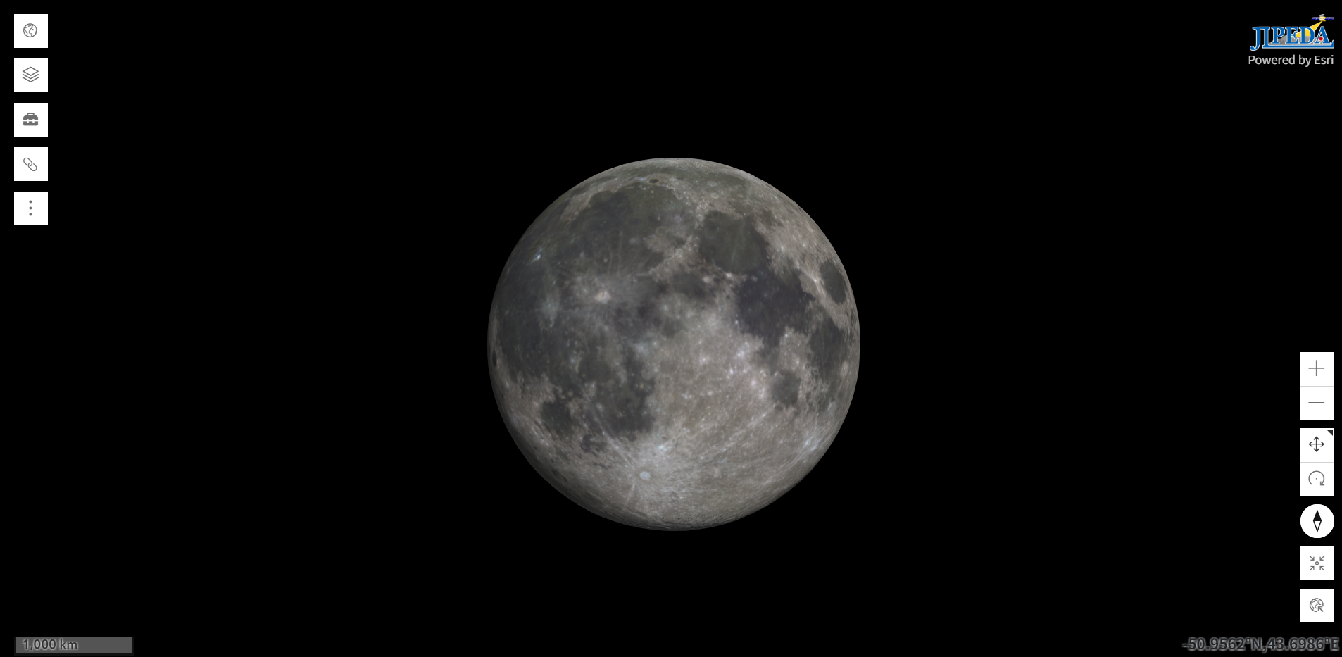
Area	Description	Example Functions
①	Buttons for basic operations	Switching views, layer operations, toolbox, share link, help, etc.
②	Buttons for view navigation	Zooming in and out, changing the viewpoint (oblique view), navigating to specified coordinates, etc.
③	Information display area that does not require button operations	Scale bar, color bar, coordinate display, display of physical quantities, etc.
④	Map display area	Layer popups

2.2. Basic Operations

Basic application functions can be accessed using the buttons in Area ① of the main screen described in Section 2.1.

Switch Views
Layer list
Toolbox
Share
Others

2.2.1 Switching Views

JAXA Virtual Planet provides the seven views listed below. View ① is the default view. The view can be changed using the “Switch Views” button. Views ① to ④ are created when the application starts and are retained in memory, so the state of each view is preserved after switching to another view. Views ⑤ to ⑦ are created and deleted as needed because of memory limitations, so they are reset when the user switches to another view.

View	Coordinate System
① 3D Globe	Geographic coordinate system: GCS_MOON_2000
② Equidistant Cylindrical 3D	Projected coordinate system: Simple Cylindrical projection SIMPLE_CYLINDRICAL_MOON
③ North Polar Stereographic 3D	Projected coordinate system: Polar Stereographic projection PolarStereographic_Moon
④ South Polar Stereographic 3D	Projected coordinate system: Polar Stereographic projection PolarStereographic_Moon
⑤ Equidistant Cylindrical 2D	Projected coordinate system: Simple Cylindrical projection SIMPLE_CYLINDRICAL_MOON
⑥ North Polar Stereographic 2D	Projected coordinate system: Polar Stereographic projection PolarStereographic_Moon
⑦ South Polar Stereographic 2D	Projected coordinate system: Polar Stereographic projection PolarStereographic_Moon

2.2.2 Layer list

When JAXA Virtual Planet starts, only the basemap is displayed. Other layers can be added as needed using the “Layer list” button described in Section 2.2, “Basic Operations.” The layer operations are described below.

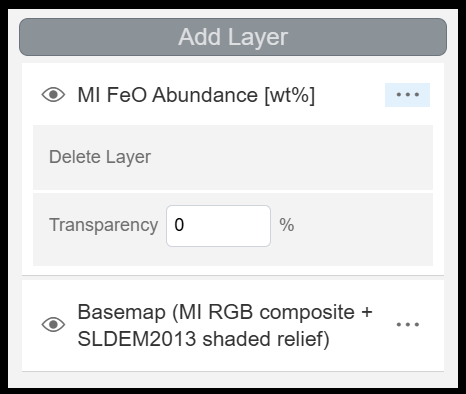
Part	Description
Add Layer	Adds selected layers to the view from the list of available layers. Multiple layers can be selected and added at once using Ctrl + left-click.
Drag	Changes the display order of the layers by dragging them.
	Left-click to toggle the visibility of the selected layer.
Delete Layer	Removes the selected layer. Note: The basemap cannot be removed.
Transparency	Sets the transparency of the selected layer.

2.2.3 Toolbox

The following functions are available from the “Toolbox” button described in Section 2.2, “Basic Operations.” For details of each function, refer to Section 2.6.

Distance Measurement
Area Measurement
Elevation Profile*
Memo*
Print*
Custom Visualization*
Download*
Add Point by Coordinates*
Subsolar/Sub-Earth points*
Search by Name

*Functions marked with an asterisk are available in Advanced mode only.

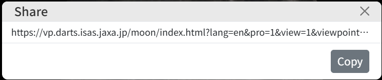
Clicking the “Share” button provides a URL that reproduces the current view. This URL can be used to share the view with others. Note that if the URL in the address bar is shared instead, the initial view will be displayed.

2.2.5. Others

Documentation on operations, physical quantities, and related information can be opened in a new tab using the “Help” button, indicated by a question mark (“?”). Clicking the “Homepage” button, indicated by a house icon, opens the homepage in a new tab. The “Switch Languages” and “Switch Mode” buttons can be used to switch between Japanese and English and between Basic and Advanced modes, respectively.

	Opens the user guide in a new tab.
	Opens the homepage in a new tab.
	Switches between Japanese and English. Note: The application restarts after the language setting is changed.
	Switches between Basic and Advanced modes. Note: The application restarts after the mode setting is changed.

Opens the user guide in a new tab.

Opens the homepage in a new tab.

Switches between Japanese and English.

Note: The application restarts after the language setting is changed.

Switches between Basic and Advanced modes.

Note: The application restarts after the mode setting is changed.

The map view can be controlled using the buttons in Area ② of the main screen or by operating directly on the map in Area ④. The functions of each button are shown in the figure below. The left buttons are for 2D views, and the right buttons are for 3D views.

Panning is the default mouse-drag operation. In 3D views, however, the dragging operation can be switched between panning and vertical view rotation. Vertical rotation enables an oblique view. Other view navigation operations assigned to mouse and touch gestures are listed below.

Mouse Operation	Function
Drag	Pan Vertical rotation^*1
Double-click	Zoom in
Ctrl + double-click	Zoom out
Scroll up	Zoom in
Scroll down	Zoom out
Right-click + drag	3D rotation
Shift + left-click + drag	Zoom to the area specified by dragging^*2
Arrow keys	Pan in four directions
N	North up
W/A/S/D keys	Rotate in the corresponding directions^*3
+	Zoom in
-	Zoom out

Touch Operation	Function
Swipe Multi-touch swipe	Pan
Double-tap	Zoom in
Pinch in/out	Zoom in/out
Two-finger rotation	Rotate

*1 In 2D views, only panning is available. In 3D views, panning and vertical rotation can be toggled using button.

*2 Available only in 2D views.

*3 In 3D views, the rotation directions assigned to the A and D keys are reversed.

2.3.1. Reset View

Clicking “Reset View” resets the viewpoint to its initial position when JAXA Virtual Planet was started.

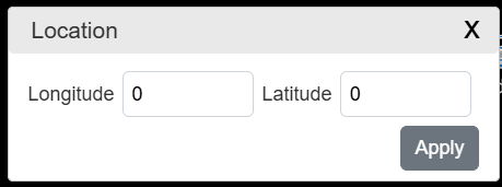
Clicking “Enter lat, lon” displays the latitude and longitude at the current center of the view. Enter any coordinates and click the “Apply” button to move the view so that the specified coordinates are at the center of the view. The zoom level remains unchanged. Longitude can be entered in either the 0° to 360° or −180° to 180° format. Out-of-range values cannot be entered.

2.4. Information Display

This section describes the information displayed in Area ③.

2.4.1. Scale Bar

A scale bar for the current view is displayed in the lower-left corner of the screen. In a 3D view, it shows the scale at the center of the map.

2.4.2. Latitude / Longitude and Physical Quantity Display

After the mouse pointer remains stationary for 0.5 seconds, the latitude and longitude at that position are displayed in the lower-right corner, and the physical quantity is displayed in the lower-left corner next to the scale bar.

Physical quantities are displayed only for image layers. They are not displayed for auxiliary layers such as graticules and place names, or for feature layers (e.g., LRS or SP).

2.4.3. Color Bar

When the layer displayed on top is an image layer or the “Mare unit age [Gyr]” layer, a color bar for the displayed physical quantities is shown in the lower-left corner.

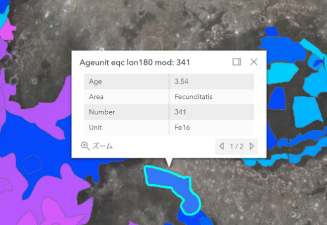
When the screen is clicked while one or more layers are displayed, related information appears in a popup. Information for the topmost layer is displayed first, and users can select another layer in the popup.

2.6. Feature-specific Operations

This section describes how to use individual functions. These operations are accessed from the “Toolbox” in Area ① of the main screen.

2.6.1. Distance Measurement

The distance between selected points can be measured by selecting “New measurement” and clicking two points on the map.

2.6.2. Area Measurement

The area of any polygon can be measured by selecting “New measurement” and clicking points on the map to define the polygon.

2.6.3. Elevation Profile (Advanced mode only)

An elevation profile along a selected line can be generated by selecting “New profile” and clicking points on the map to define the line. The measurement data can be downloaded in CSV format from “Toolbox” > “Download”.

2.6.4. Memo (Advanced mode only)

Using “Memo”, you can draw a shape on the map and attach a text note to it. The note is saved in a dedicated Memo layer.

2.6.5. Print (Advanced mode only)

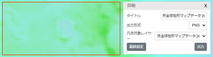
An image or PDF of a selected area of the current view can be output. The output is a capture of the displayed view rather than the original image data.

2.6.6. Custom Visualization (Advanced mode only)

“Custom Visualization” is the operation of defining a function filter for an image layer to generate a layer with a different visualization. “Custom Visualization” cannot be applied again to a Custom Visualization layer. However, a color map can be applied to a layer generated by the “Raster Calculator.”

The following three types of Custom Visualization are supported.

Operation type	Definition
Color map	Maps pixel values according to a color map and displays a single-band raster as a grayscale or gradient image. As preprocessing, a Min/Max stretch or histogram equalization is applied, and the pixel values are converted to a range of 0–255.
RGB Composite	Combines three raster bands into a single RGB raster.
Raster Calculator	Calculates a raster from a mathematical expression based on raster bands.

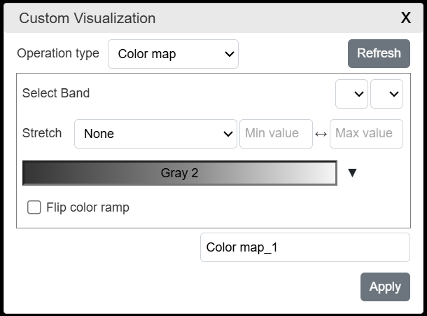
The operating procedure is described below. The Custom Visualization settings screen is divided into Parts ① to ③.

Part	Description
①	Select “Color map”, “RGB Composite”, or “Raster Calculator” from the list.
②	Detailed settings corresponding to the function selected in Part ① are displayed.
③	Enter the name of the output layer. If the specified name is the same as that of an existing layer, the existing layer is overwritten.

The settings for each type of Custom Visualization are described below.

	Description
Color map	1. “Select Band”: Select an image layer from the list. A list of bands in the selected layer is displayed. Select a band from this list. 2. Specify the stretch to be applied to the output. Select “None”, “Min/Max”, or “Histogram Equalization”. - None: The pixel values are converted to the range of 0–255 using the minimum and maximum pixel values of the layer. - Min/Max: The specified pixel-value range is converted to the range of 0–255. Values outside the specified range are assigned the NoData value (−9999) and displayed as transparent. - Histogram Equalization: After histogram equalization is applied, the pixel values are converted to the range of 0–255 using the minimum and maximum pixel values of the layer. 3. Select the color map to be applied from the list of color maps. Grayscale is selected by default.
RGB Composite*	1. “Select Band”: Select the bands to be assigned to the red, green, and blue channels from the list of image layers and the list of bands in each selected layer. 2. To limit the output range of each band, specify the minimum and maximum values. Values outside the specified range are replaced with the corresponding minimum or maximum value.
Raster Calculator*	Assign the bands specified under “Select Band” to variable names and display a layer generated by raster calculation. Up to three variables (a, b, and c) can be used in a calculation. Enter the mathematical expression to be executed in the text box at the bottom of the screen. The available operators conform to the following specification: https://pro.arcgis.com/en/pro-app/latest/help/analysis/raster-functions/calculator-function.htm To apply an exponential or logarithmic function to a band before passing it to the expression, select the function from the list to the right of the band name.

Description

Color map

1. “Select Band”: Select an image layer from the list. A list of bands in the selected layer is displayed. Select a band from this list.

2. Specify the stretch to be applied to the output. Select “None”, “Min/Max”, or “Histogram Equalization”.

- None: The pixel values are converted to the range of 0–255 using the minimum and maximum pixel values of the layer.

- Min/Max: The specified pixel-value range is converted to the range of 0–255. Values outside the specified range are assigned the NoData value (−9999) and displayed as transparent.

- Histogram Equalization: After histogram equalization is applied, the pixel values are converted to the range of 0–255 using the minimum and maximum pixel values of the layer.

3. Select the color map to be applied from the list of color maps. Grayscale is selected by default.

RGB Composite*

1. “Select Band”: Select the bands to be assigned to the red, green, and blue channels from the list of image layers and the list of bands in each selected layer.

2. To limit the output range of each band, specify the minimum and maximum values. Values outside the specified range are replaced with the corresponding minimum or maximum value.

Raster Calculator*

Assign the bands specified under “Select Band” to variable names and display a layer generated by raster calculation. Up to three variables (a, b, and c) can be used in a calculation. Enter the mathematical expression to be executed in the text box at the bottom of the screen. The available operators conform to the following specification:

https://pro.arcgis.com/en/pro-app/latest/help/analysis/raster-functions/calculator-function.htm

To apply an exponential or logarithmic function to a band before passing it to the expression, select the function from the list to the right of the band name.

* These functions are available only for the following three layers: MI reflectance, MI FeO Abundance [wt%], and MI TiO2 Abundance [wt%].

2.6.7. Download (Advanced mode only)

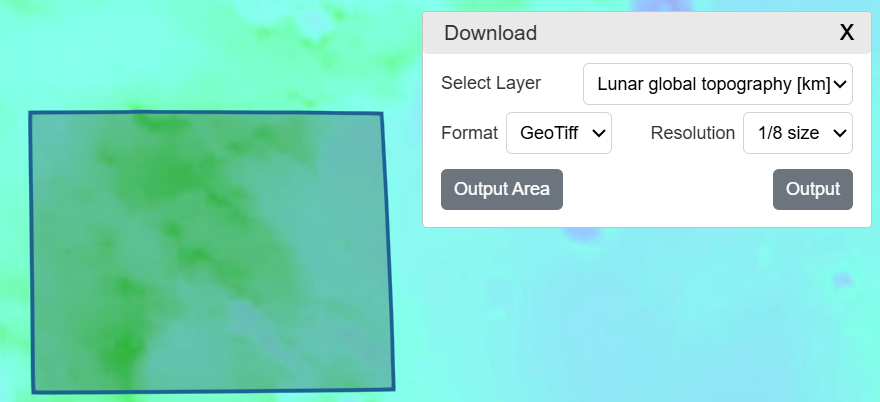
This section describes how to download data for a selected area of a selected layer.

Item	Description
Select Layer	Select the layer to be downloaded from the layers that have been added to the “Layer list.”
Format	Select the output format. The available formats depend on the layer type. - Image layers: GeoTIFF - SP/LRS layers: Shapefile or CSV
Resolution	Select Original, 1/2 size, 1/4 size, or 1/8 size. This option is available only when an image layer is selected for download.
Output Area	Specify the output area as a rectangle. Clicking the “Output Area” button activates rectangle input mode, allowing a rectangle to be drawn on the screen.
Output	Starts the download process. When processing is complete, a download link appears at the bottom of the screen. The maximum downloadable image size (rows × columns) is 4,100 × 15,000 pixels, depending on the selected resolution. A maximum of 2,000 SP/LRS records can be downloaded.

2.6.7.1. SP Data Output Format

The Spectral Profiler (SP) observation data fields included in Shapefile and CSV output are shown below.

Shapefile Format

Field Name	Description	Remarks
FID	Shapefile-specific field
Shape	Shapefile-specific field
Revo_num	Orbital revolution number	REVOLUTION_NUMBER in the LBL file
Strip_num	Strip number within the revolution	STRIP_SEQUENCE_NUMBER in the LBL file
Scene_num	Scene number within the strip	SCENE_SEQUENCE_NUMBER in the LBL file
Serial_num	Sequential number within the same Scene_num, Strip_num, and Revo_num combination
Spc_url	Data URL
Lbl_url	LBL URL
Thumbnail	Thumbnail image URL

CSV Format (SP_ref.csv)

Field Name	Description	Remarks
Revo_num	Orbital revolution number	REVOLUTION_NUMBER in the LBL file
Strip_num	Strip number within the revolution	STRIP_SEQUENCE_NUMBER in the LBL file
Scene_num	Scene number within the strip	SCENE_SEQUENCE_NUMBER in the LBL file
Serial_num	Sequential number within the same Scene_num, Strip_num, and Revo_num combination
Spc_url	Data URL
Lbl_url	LBL URL
Thumbnail	Thumbnail image URL
Longitude	Longitude
Latitude	Latitude
Ref5126	Diffuse reflectance value at a wavelength of 512.6 nm	296 fields The wavelength of each band in nanometers is obtained by dividing the four- or five-digit number following Ref by 10.
・・・
Ref25879	Diffuse reflectance value at a wavelength of 2587.9 nm

CSV Format (SP_rad.csv)

Field Name	Description	Remarks
Revo_num	Orbital revolution number	REVOLUTION_NUMBER in the LBL file
Strip_num	Strip number within the revolution	STRIP_SEQUENCE_NUMBER in the LBL file
Scene_num	Scene number within the strip	SCENE_SEQUENCE_NUMBER in the LBL file
Serial_num	Sequential number within the same Scene_num, Strip_num, and Revo_num combination
Spc_url	Data URL
Lbl_url	LBL URL
Thumbnail	Thumbnail image URL
Longitude	Longitude
Latitude	Latitude
Rad5126	Spectral (diffuse) radiance value at a wavelength of 512.6 nm	296 fields The wavelength of each band in nanometers is obtained by dividing the four- or five-digit number following Rad by 10.
・・・
Rad25879	Spectral (diffuse) radiance value at a wavelength of 2587.9 nm

2.6.7.2. LRS Data Output Format

The Lunar Radar Sounder (LRS) observation data fields included in Shapefile and CSV output are shown below.

Field Name	Description	Remarks
FID	Shapefile-specific field	Not included in CSV downloads.
Shape	Shapefile-specific field	Not included in CSV downloads.
Lon_start	Longitude of the start point of the line segment
Lat_start	Latitude of the start point of the line segment
Lon_end	Longitude of the end point of the line segment
Lat_end	Latitude of the end point of the line segment
Img_url	Data URL
Lbl_url	LBL URL
Thumbnail	Thumbnail image URL

2.6.8. Subsolar/Sub-Earth Points (Advanced mode only)

Displays the subsolar point and sub-Earth point on the lunar surface at a specified date and time. The points are displayed in the Subsolar/Sub-Earth Points feature layer.

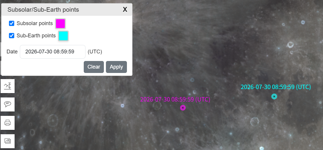
Item	Description
Subsolar Points / Sub-Earth Points	Displays the subsolar point and/or sub-Earth point selected using the checkboxes.
Date	Specifies the date and time for which the subsolar and sub-Earth points will be created.
Clear	Deletes all points.
Apply	Creates the subsolar and sub-Earth points at the specified date.

2.6.9. Search by Name

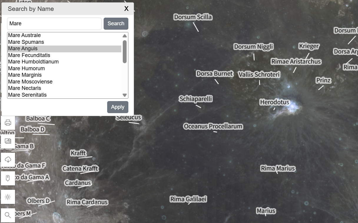
Displays a list of lunar Nomenclature names based on a keyword search. Select an entry and click the “Apply” button to move to that location.

Analysis example from JAXA Virtual Planet

Perform many different types of analyses on JAXA Virtual Planet. An example of an analysis via band ratioing using MI reflectance data can be downloaded from the following link.

Open the data analysis procedure manual (PDF)